NumPy Blog 2
Learning objectives of this blog -
* Creating 1-D and 2-D arrays with the in-built methods of NumPy library like -->
ones( ), arange( ), linspace( ), copy( ), reshape( )
* Attributes of NumPy, their usage and purpose
* Understanding some other built-in methods of NumPy


Code 4


Example 1


Learning objectives of this blog -
* Creating 1-D and 2-D arrays with the in-built methods of NumPy library like -->
ones( ), arange( ), linspace( ), copy( ), reshape( )
* Attributes of NumPy, their usage and purpose
* Understanding some other built-in methods of NumPy
All the programs written in the code editor window along with the output has to be maintained in the IP Register along with the Text highlighted in blue.
Some more code examples

ones( )
The default data type of this method is float. (which means each element that is '1' will have a decimal dot suffixed to it.
Syntax -- <numpy_object>.ones( [ no_of_rows ] , [no_of_columns] , dtype = 'int' )
Code Ex. 1 import numpy as np
print(np.ones(5))
# in the above code there is only one argument value '5', so no_of_rows = 1(default) and no_of_columns = 5.
Output = [ 1. 1. 1. 1. 1. ]
Code ex. 2 import numpy as np
print(np.ones([2, 5]))
#in the above code the dimension of the matrix is of 2 rows and 5 columns.
#in the above code dtype argument is assigned to value ‘int’ which means all the element values which is 1, of this matrix will be integer and will no more appear as a float.
Output - [ 1 1 1 1 1 ]
[ 1 1 1 1 1 ]
Some more code examples

arange( )
Syntax- <object_name>.arange(start_value, stop_value, jump_value) # default data type is int
Code 1
print
Output - [ 0 1 2 3 4 5 6 7 8 9 ]
Q^ in the above code why 10 is not being displayed?
1
|
2
|
3
|
4
|
5
|
Start Value
|
Current Value
|
Start value<Stop value if yes
|
print
|
Jump Value = Current value + 1
|
0
|
0
|
0<10 yes
|
[ 0 ]
|
0 + 1 =1
|
1
|
1<10 yes
|
[ 0 1 ]
|
1 + 1 =2
| |
2
|
2<10 yes
|
[ 0 1 2 ]
|
2 + 1 =3
| |
3
| ||||
.
| ||||
.
| ||||
9
|
9<10 yes
|
[0 1 2 ….. 9 ]
|
9 + 1 =10
| |
10
|
10<10 no X
|
x
|
x
|
The condition becomes false and so execution stops and loop is terminated,
so that is why 10 is not displayed as the last value of the array but 9 is.
Code 3
M-D
Code 1
for j in numpy.arange(1):
print(i, j)
The Working Mechanism of the above code
Step1
|
Step2
|
Step3
|
Step4
|
Step5
|
Step6
|
Step7
|
Step8
|
Step9
|
i
|
i<13 (if yes continue else exit from loop)
|
j.
|
j<1 (if yes continue else exit from loop)
|
print(i,j)
|
j++
|
loop to j condition check
(step 4)
|
i++
|
loop to i condition check
(step 2)
|
11
|
11<13 yes
|
0
|
0<1 yes
|
11 0
|
1
|
jump to Step 4
| ||
1<1 no jump to Step 8
|
12
|
Jump to Step 2
| ||||||
12<13 yes
|
0
|
0<1 yes
|
12 0
|
1
|
jump to Step 4
| |||
1<1 no jump to Step 8
|
13
|
Jump to Step 2
| ||||||
13<13 no (exit the loop)
|
X
|
X
|
X
|
X
|
X
|
X
|
X
|
In the above code variable i and j reaches till the value 13 and 1 respectively but do not execute for these values. (because the condition becomes false for these values)
So the output of the program is 11 0
12 0
But the last value of variable i and j is 13 and 1 respectively.
Code 2
Loop 1 (Outer Most)
|
Loop 2 (Inner)
|
Loop 3
|
Output
|
.arange(1)
|
-
|
-
|
0
|
.arange(1)
|
.arange(1)
|
-
|
0 0
|
.arange(1)
|
.arange(1)
|
.arange(1)
|
0 0 0
|
.arange(1,2)
|
-
|
-
|
1
|
.arange(1,2)
|
. arange(1)
|
-
|
1 0
|
.arange(1,2)
|
.arange(1,2)
|
-
|
1 1
|
.arange(1,2)
|
.arange(1,2)
|
.arange(1,2)
|
1 1 1
|
.arange(1,2)
|
.arange(1,2)
|
.arange(1)
|
1 1 0
|
.arange(1,2)
|
.arange(1)
|
.arange(1)
|
1 0 0
|
In all of the above examples all of the loops have 1 element value so there is always one single row output.
| |||
Code 3
.arange(1,3)
|
-
|
-
|
1
2
|
.arange(1,3)
|
.arange(1)
|
-
|
1 0
2 0
|
.arange(1,3)
|
.arange(1)
|
.arange(1)
|
1 0 0
2 0 0
|
.arange(1,3)
|
.arange(1,2)
|
-
|
1 1
2 1
|
.arange(1,3)
|
.arange(1,2)
|
.arange(1,2)
|
1 1 1
2 1 1
|
.arange(1,3)
|
.arange(1,2)
|
.arange(1)
|
1 1 0
2 1 0
|
?
|
?
|
?
|
1 0 1
2 0 1
|
In all of the above examples
The outer loop has more than one element values but at the same time all the inner loops have only 1 element value, so the output has 2 rows filled with the respective loop’s element values.
| |||
Code 4
.arange(1, 3)
|
.arange(1,3)
|
-
|
1 1
1 2
2 1
2 2
|
The working mechanism for the above code is below --
Step1
|
Step2
|
Step3
|
Step4
|
Step5
|
Step6
|
Step7
|
Step8
|
Step9
|
.arange(1,3)
Loop1
|
condition
loop1 current value<3
if yes next step
if no then exit
|
.arange(1,3)
Loop2
|
condition
loop2 current value<3
if yes next step
if no then Step 8
|
print(loop1, loop2)
|
increase loop2 by 1
|
Jump to step 4
|
increase loop1 by 1
|
Jump to Step 2
|
1
|
1<à
|
1
|
1<
yes - next step ---
|
1 1
|
1+1 = 2
|
jump to Step 4
| ||
2
|
2<
yes - next step ---
|
1 2
|
2+1=3
|
jump to Step 4
| ||||
3
|
3<
no – jump to step 8
|
Skip
|
Skip
|
Skip
|
1+1=2
|
Jump to Step2
| ||
2
|
2<à
|
1
|
1<
|
2 1
|
1+1 = 2
|
jump to Step 4
| ||
2
|
2<
yes - next step -
|
2 2
|
2+1=3
|
jump to Step 4
| ||||
3
|
3<
no – jump to step 8
|
Skip
|
Skip
|
Skip
|
2+1=3
|
Jump to Step2
| ||
3
|
3<
|
X
|
X
|
X
|
x
|
X
|
X
|
X
|
Code 5
.arange(1,3)
|
.arange(1,3)
|
.arange(1)
|
1 1 0
1 2 0
2 1 0
2 2 0
|
.arange(1,3)
|
.arange(1,3)
|
.arange(1,2)
|
1 1 1
1 2 1
2 1 1
2 2 1
|
.arange(1,3)
|
.arange(1,3)
|
.arange(1,3)
|
1 1 1
1 1 2
1 2 1
1 2 2
2 1 1
2 1 2
2 2 1
2 2 2
|
Some more code examples are -
linspace( )
** This function is somewhat like arange( ) but the difference is this method uses interval gaps instead of jump values.
Syntax
#total_values = total number of data in the range including the start and stop value
#equalgap = ( stop_value - start_value )
#default data type is float.
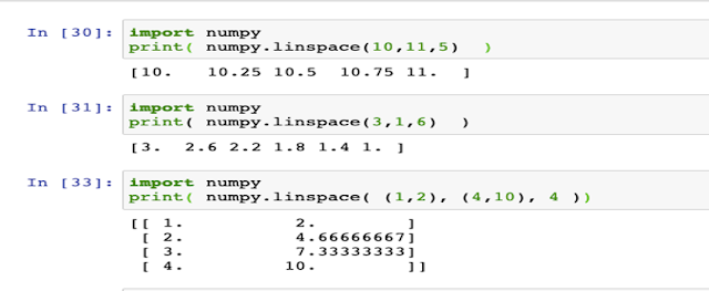
Code 1
print(“Five data from 10 to 11 at equal gap or difference are ”)
print( numpy.linspace(10,11,5) )
# total values = 5
(Which means a data range like
# stop_value – start_value = 11-10 = 1
# equalgap / the exact difference between each two values or the x = 11-10/5-1
x =
x = 0.25
Now, the data range = [ 10 10+0.25 10+0.25+0.25 10+0.25+0.25+0.25 11 ]
Final Output =
Five data from 10 to 11 at equal gap or difference are
[ 10. 10.25 10.50 10.75 11. ]
Code 2
print(“Six data from 3 to 1 at equal gap or difference are ”)
print( numpy.linspace(3,1,6) )
# total values = 6
(Which means a data range like 3 3-x 3-x-x 3-x-x-x 3-x-x-x-x 1 )
# stop_value – start_value = 3-1 = 2
# equalgap / the exact difference between each two values or the x = 3-1 / 6-1
x = 2 / 5
x = 0.4
Now, the data range = [ 3 3-0.4 3-0.4-0.4 3-0.4-0.4-0.4 3-0.4-0.4-0.4-0.4 1 ]
Final Output =
Six data from 3 to 1 at equal gap or difference are
[ 3. 2.6 2.2 1.8 1.4 1. ]
Code 3
print(“4 data in an array in the first column between 1 to 4 and in
the second column between 2 to 10 at equal gap or difference are ”)
print
When linspace( ) is specified with pair of range values in arguments then data range appears in matrix
Then the definition of start_value and stop_value changes.
Here in the matrix to be formed the Column 1 data range = 1 to 4 and Column 2 data range = 2 to 10
# total values = 4 in each data range
Which means a data range like
1+x 2+y
1+x+x 2+y+y
4 10 ]
For Column 1
# stop_value – start_value = 4-1 = 3
# equalgap / the exact difference between each two values or the x = 4-1/4-1
x = 3/3
x = 1
Now, the data range = [ 1.
1.+1.
1.+1.+1.
4. ]
For Column 2
# stop_value – start_value = 10-2 = 8
# equalgap / the exact difference between each two values or the y = 10-2/4-1
y = 8/3
y = 2.6667
Now, the data range = [ 2.
2.+2.6667
2.+2.6667+2.6667
10. ]
Final Output =
[ [ 1. 2. ]
[ 2. 4.66666667 ]
[ 3. 7.33333333 ]
[ 4. 10. ] ]
copy( )
import numpy
x
y=numpy.copy(x) #copying the structure and data of array ‘x’ to ‘y’
print(y)
In the second code example 'y' is an array variable which is a copy of the array 'x' and is being increased by value 10. Which means that each element of the array will be increased by 10. And thats is reflected in the output too.
reshape( )
Syntax - <array_variable>.reshape( no_rows, no_col )
Eg -
print(x.reshape(3,2)) # 3x2 = 6
** copy( ) and reshape( ) needs a predefined array variable as its argument.
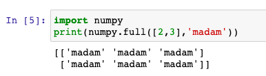
full( )
Syntax
shape
fill_value : [bool, optional] Value to fill in the array (Compulsory)
dtype : [optional, float(by Default)] Data type of returned array.
In the above examples shape is when specified as one value in the argument of this function then it becomes total number of columns and number of rows remain 1 (as default).
When 2 values are specified as matrix dimension in the argument of this function then the first value is number of rows and second value is number of columns.
Example 2
In the above example the fill value is a boolean value True for the matrix of 3x3 and is shown in the output too.
Example 3
In the above example the fill value is a string value 'madam' for a matrix of 2x3 and is reflected in the output too.
Some other methods of Numpy
all( )
This function returns “true” if all items/elements in the array are other than 0, even if one element is 0 then this function returns “false” as an output.
When in the array
|
Will Return
|
Any one element is 0
|
False
|
All the elements are 0
|
False
|
None of the elements are 0
|
True
|
Empty array
|
True
|
tolist( )
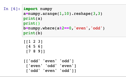
where( )
Syntax – <numpy_object>.where(array_condition, true statement, false statement)
Array_condition – is the condition specified on the array
True_statement – is the output which we want to see when the condition is satisfied
False_statement – is the output which we want to see when the condition is dissatisfied
In the above example a%2 means each element of array a is divided by 2 and the remainder is collected
Now a%2==0 means that the remainder of each element after being divided by 2 is checked whether is qual to 0 or not (even number)
If the condition is true that means if the element is even then the true_statement will be displayed at those elements places.
Which means in the above statement the true_statement value is 0 so each element in the array which is even will be replaced by 0 and each element which is odd will be replaced by 1 because that is the false_statement value.
Code 2
In the above example the elements of the array a is being checked for even number and if the element is even the true statement is 'even' and the false statement is 'odd'.
Code 3
In the above example the array a elements are being checked for even number and if the element is an even number then the value being displayed in place of those elements is '0' as true statement otherwise the original value of the array is displayed because the false statement is the array 'a' itself.
Code 4
In the above example the odd numbers have been increased by 2 and the even numbers have been replaced by 0.
Code 5
Attributes of NumPy
Library in a language has a collection of built-in modules / packages / methods / attributes to perform various task in order to achieve a desired output. Attributes are predefined or built-in elements of a module which are called or accessed to perform a special task or get a desired output.
mgrid[ ]
Syntax - <object_name>.mgrid[ dimesion1_values , dimension2_values, ……]
dimension1_values = [start_value : stop_value]
start_value = is the number from which data value will be generated
stop_value = the data value will be generated upto one less than the stop_value
In the above example In [49] : a matrix is being created with a NULL value because the data range for this matrix / array variable ‘a’ start_value data is 1 and stop_value data is one less than the stop_value which is 1-1=0.
So no data will be generated by this mgrid[ ] attribute and the output will be an empty array.
In the above example In [50] : a matrix of 2 Dimensions or subgrids is being created but with a NULL value in each dimension or subgrid because the data range for this array variable ‘a’ for both the subgrid start_value data is 1 and stop_value data is one less than the stop_value which is 1-1=0.
So no data will be generated by this mgrid[ ] attribute and the output will be an empty array.
I
So there will be 1 data generated by the mgrid[ ] and the data value is ‘0’.
In the above example In[54]:
For 1
start_value data = 0 as it is not given so the default is start_value data is 0 [ no start_value : 1 ]
stop_value data = 0 as the given stop_value is 1, so 1-1=0
So there will be 1 data generated by the mgrid[ ] and that data value is [ 0 ]
For 2
start_value data = 0 as it is not given so the default is start_value data is 0 [ no start_value : 1 ]
stop_value data = 0 as the given stop_value is 1, so 1-1=0
So there will be 1 data generated by the mgrid[ ] and that data value is [ 0 ]
So the Final Output for the Main Grid
Grid 1
Grid 2
]
In the above example In[56]: a matrix of 1 dimension or subgrid is created where
Start_value data = 1 as given
Stop_value data = 2-1 = 1 as the given stop_value is 2.
So there will be 1 data generated by the mgrid[ 1 : 2 ]= and that data value is [ 1 ]
In the above example In[57]: a matrix of 2 dimensions or subgrids are created where
For 1
start_value data = 1 as given
stop_value data = 1 as the given stop_value is 2, so 2-1=1
So there will be 1 data generated by the mgrid[ 1 : 2 ] and that data value is [ 1 ]
For 2
start_value data = 1 as given
stop_value data = 1 as the given stop_value is 2, so 2-1=1
So there will be 1 data generated by the mgrid[ 1 : 2 ] and that data value is [ 1 ]
So the Final Output for the Main Grid [
Grid 1 [ [ 1 ] ]
Grid 2 [ [ 1 ] ]
]
See some more code examples
2. version
import numpy
print(numpy.version.version)
OR
import numpy
print(numpy._version_)
3. shape
import numpy
a=numpy.arange(1,11)
print(a)
print(a.shape)
Output
(10,) 10 columns 1 row
import numpy
a=numpy.mgrid[1:4]
print(a)
print(a.shape)
(3,) 3 columns 1 row
See some more code examples
That's all for this blog page !!! Raise your doubts either in the comment boxor reach me at my inbox!!
Stay Safe Stay Healthy!!!
No comments:
Post a Comment